Biology Speaks Code: A Crash Course in Computational Biology
What computational biology actually covers, and where idgence’s own work — docking, molecular dynamics, and machine learning — fits inside it.
A modern DNA sequencer can read a human genome — about 3 billion letters — in under a day. No team of scientists will ever read that output letter by letter. Somewhere between the raw data and a discovery, a computer has to do most of the looking. That gap is what computational biology exists to fill.
So what is it, exactly?
The U.S. National Library of Medicine’s standard definition is blunt and useful: computational biology is the field concerned with developing techniques to collect and manipulate biological data, and using that data to make biological discoveries or predictions. In practice, that means writing algorithms, building statistical models, and running simulations that stand in for experiments too large, too slow, or too expensive to run directly in a lab.
It’s a big tent. The field doesn’t have one method or one kind of problem — it has a shared habit of turning biological questions into computational ones.
A map of the territory
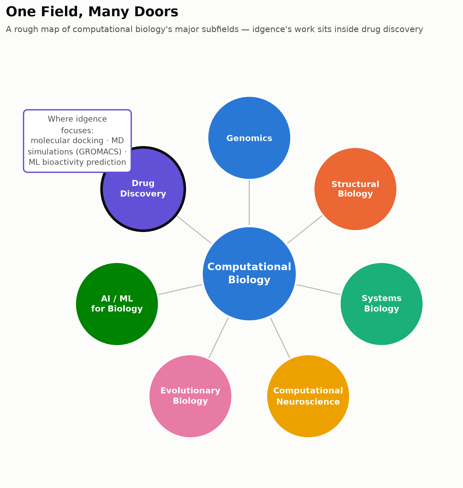
UC Berkeley’s Center for Computational Biology groups its own research into several major areas, and the list is a reasonable sketch of the field as a whole:
- Genomics — reading and interpreting DNA and RNA sequences at scale
- Structural biology — predicting and analyzing the 3D shapes of proteins and other biomolecules
- Systems biology — modeling how genes, proteins, and pathways interact as a network rather than in isolation
- Computational neuroscience — simulating neural circuits and brain function
- Evolutionary biology — tracing how genomes and populations change over time
- AI/ML for biology — applying machine learning to prediction problems across all of the above
- Drug discovery — using computation to find and refine therapeutic molecules before they ever touch a lab bench
Most research groups — idgence included — don’t live in just one of these boxes. A single drug-discovery project might touch structural biology (the target protein’s shape), systems biology (what pathway it sits in), and AI/ML (predicting which candidate molecules are worth testing).
Where idgence’s work sits
idgence’s own research lives mainly in that last category — computational drug discovery — using three tools in combination:
- Molecular docking, which predicts how a small molecule physically fits into a protein’s binding pocket, and roughly how tightly it holds on.
- Molecular dynamics (MD) simulations, typically run with software like GROMACS, which test whether a predicted docking pose actually holds up over time under realistic physical conditions, rather than just looking good in a single static snapshot.
- Machine learning models for bioactivity prediction, which learn from existing data to flag which molecules, out of thousands or millions of candidates, are worth the computational or experimental effort to check further.
This isn’t abstract for this site — it’s already what idgence’s published work looks like. The virtual screen that found a novel Keap1 inhibitor for neurodegeneration combined docking and MD simulation to narrow 14,492 marine compounds down to one candidate. The RIPK1 case study walks through the same structure-based approach as an open tutorial. And the machine-learning-guided search for RIPK1 inhibitors shows docking and MD paired directly with an ML model, rather than used on their own.
Why the map matters
None of these methods work in isolation, and none of them replace a wet lab — they replace the impossible version of a wet lab, the one where every candidate molecule gets tested by hand. Computational biology’s real job is triage: take an unmanageable search space and return a short, well-justified list.
That’s the thread running through everything on this blog. Future posts will go deeper into each piece of the toolbox — what GROMACS actually does during a simulation, how docking algorithms score a binding pose, how QSAR and newer deep-learning models predict bioactivity — building out from this map one subfield at a time. If you want a hands-on starting point before then, idgence also walks through how to select a target protein for a computational drug discovery project and runs short courses on computational drug discovery through NSU.
This post is an orientation piece for idgence’s ongoing series on in silico drug discovery. Sources: National Library of Medicine MeSH descriptor for “Computational Biology”; UC Berkeley Center for Computational Biology.